## Loading required package: ggplot2
## Loading required package: gridExtra
## Loading required package: reshape2
## Loading required package: VineCopula
## Loading required package: randtoolbox
## Loading required package: rngWELL
## This is randtoolbox. For an overview, type 'help("randtoolbox")'.
##
##
##  This is version 1.3.0 of esgtoolkit. Starting with 1.0.0, package renamed as: 'esgtoolkit' (lowercase)
##
##
# Spot variance
V0 <- 0.1372

# mean-reversion speed
kappa <- 9.5110/100

# long-term variance
theta <- 0.0285

# volatility of volatility
volvol <- 0.8010/100

# Correlation between stoch. vol and prices
rho <- -0.5483

# Intensity of the Poisson process
lambda <- 0.3635

# mean and vol of the merton jumps diffusion
mu_J <- -0.2459
sigma_J <- 0.2547/100
m <- exp(mu_J + 0.5*(sigma_J^2)) - 1

# Initial stock price
S0 <- 4468.17

# Initial short rate
r0 <- 0.0357

# ============================================================================
# SIMULATION SETUP
# ============================================================================

n <- 300
horizon <- 1
freq <- "weekly"

start_ <- start(EuStockMarkets)
end_ <- end(EuStockMarkets)
print(end_ - start_)
## [1] 7 39
freq_ <- frequency(EuStockMarkets)

# Simulation of shocks, with antithetic variates
shocks <- esgtoolkit::simshocks(n = n,
                                horizon = 8L,
                    method = "anti",
                    family = 1, par = rho,
                    start = start_, frequency=freq_)

print(start_)
## [1] 1991 130
## [1] 260
## [1] 1998 169
## [1] 1991 130
## [1] 260
## [1] 1999 129
============================================================================
VOLATILITY SIMULATION (CIR PROCESS)
============================================================================
# Vol simulation
sim_vol <- esgtoolkit::simdiff(n = n,
                   model = "CIR", x0 = V0,
                   theta1 = kappa*theta, theta2 = kappa,
                   theta3 = volvol,
                   eps = shocks[[1]],
                   start = start_,
                   frequency=freq_,
                   horizon = 8L)
print(start(sim_vol))
## [1] 1991 130
## [1] 260
## [1] 1999 130
============================================================================
ASSET PRICE SIMULATION (GBM WITH JUMPS)
============================================================================
# prices simulation
sim_price <- esgtoolkit::simdiff(n = n, start = start_,
                                 end = end_,
                                 frequency=freq_,
                     horizon = 8L,
                     model = "GBM", x0 = S0,
                     theta1 = r0 - lambda*m, theta2 = sim_vol,
                     lambda = lambda, mu_z = mu_J,
                     sigma_z = sigma_J,
                     eps = shocks[[2]])
print(start(sim_price))
## [1] 1991 130
## [1] 260
## [1] 1998 169
## [1] 1860 300
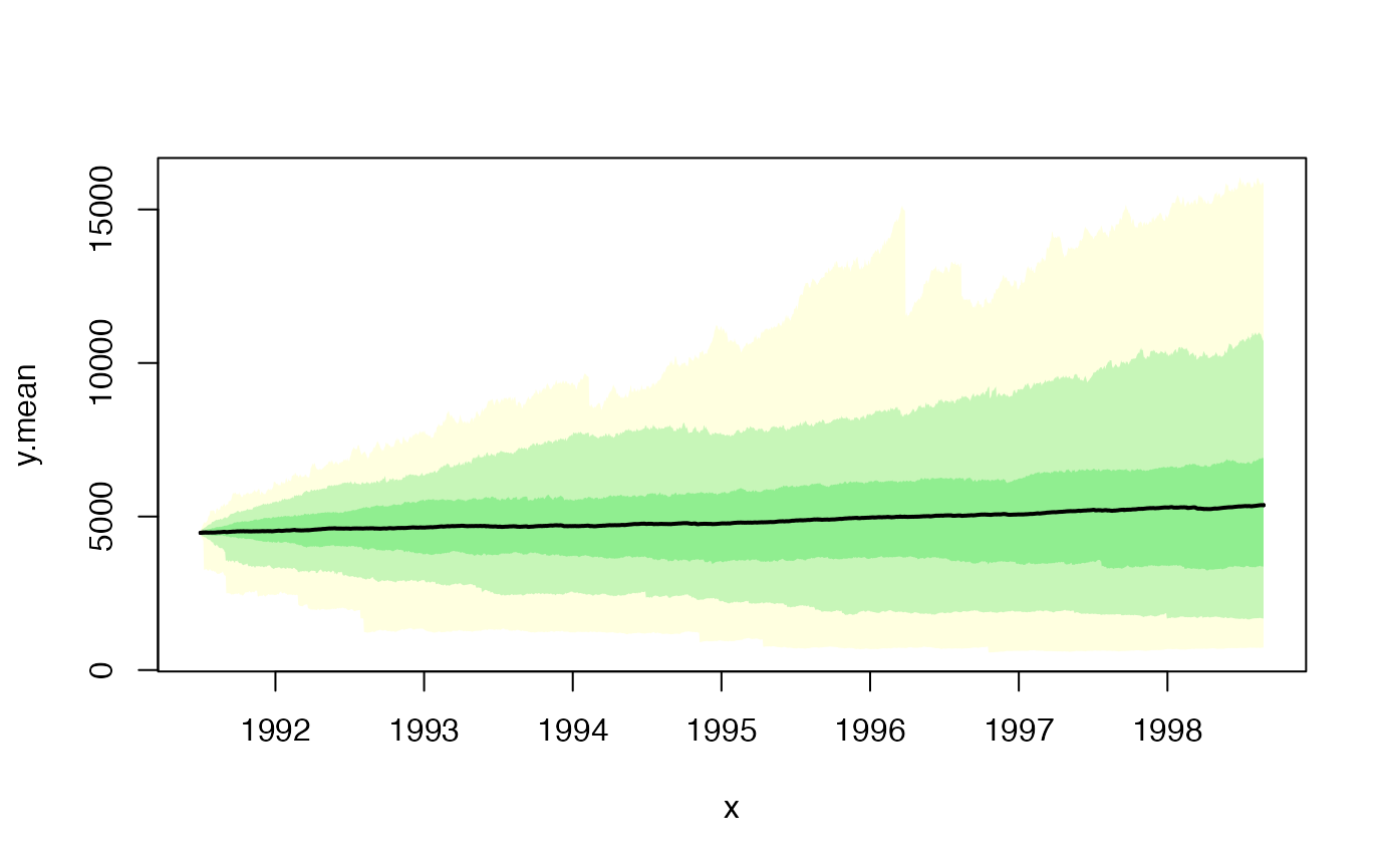
# Plot the simulated price paths
esgtoolkit::esgplotbands(sim_price)