## Loading required package: Matrix
## Loaded glmnet 4.1-10
1 - 1 Regression on Boston data set
set.seed(123)
# -------------------------
# Data
# -------------------------
X <- as.matrix(MASS::Boston[, -14]) # predictors
y <- MASS::Boston$medv # response
# Train/test split
n <- nrow(X)
idx <- sample(1:n, size = round(0.8 * n))
X_train <- X[idx, ]
y_train <- y[idx]
X_test <- X[-idx, ]
y_test <- y[-idx]
# -------------------------
# Fit model (No CV)
# -------------------------
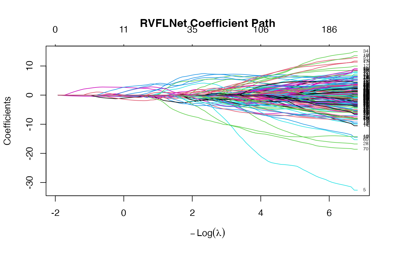
fit <- rvflnet(X_train, y_train,
n_hidden = 200,
activation = "sigmoid",
W_type = "gaussian")
plot(fit)
##
## ========================================
## RVFLNet Model (glmnet backend)
## ========================================
## Call: rvflnet(x = X_train, y = y_train, n_hidden = 200, activation = "sigmoid",     W_type = "gaussian")
## Input features: 13
## Hidden units: 200
## Total features: 213
## Activation: sigmoid
## Weight distribution: gaussian
## Seed: 1
## Input scaling: Yes
## Include original features: TRUE
## Family: gaussian
## Non-zero coefficients (min lambda): 201
## ========================================
## 6 x 3 sparse Matrix of class "dgCMatrix"
##                 s=0.10    s=0.05       s=0.01
## (Intercept) 32.7058947 50.810289  43.99161364
## crim         .          .          0.15054149
## zn           .          .          .
## indus        .          .         -0.08164812
## chas         .          .         -0.13233795
## nox         -0.1479769 -8.748572 -23.79594614
## 6 x 3 sparse Matrix of class "dgCMatrix"
##         s=0.10   s=0.05     s=0.01
## H195 .         .         .
## H196 .         .         .
## H197 .         .         .
## H198 .         .         .
## H199 .         .        -0.8183077
## H200 0.4654941 2.169695  6.0771916
##      s=0.05   s=0.03   s=0.01
## 1  28.78165 28.12491 25.65727
## 15 18.30785 18.59386 19.00496
## 17 18.94427 19.40582 19.50233
## 19 13.40825 13.04073 13.49051
## 28 13.10162 13.73416 14.60465
## 37 22.92770 22.74231 22.39807
##   s=0.05   s=0.03   s=0.01
## 3.441028 3.235019 2.937008
# -------------------------
# Fit model (CV)
# -------------------------
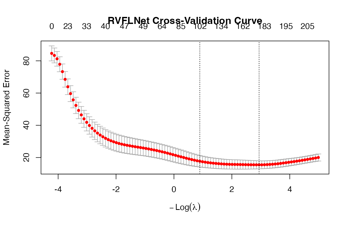
cv_model <- cv.rvflnet(
X_train, y_train,
n_hidden = 200,
activation = "sigmoid",
W_type = "gaussian",
alpha = 0.1, # elastic net mix
nfolds = 5
)
print(cv_model)
##
## ========================================
## Cross-Validated RVFLNet Model
## ========================================
## Call: cv.rvflnet(x = X_train, y = y_train, n_hidden = 200, activation = "sigmoid",     W_type = "gaussian", alpha = 0.1, nfolds = 5)
## Input features: 13
## Hidden units: 200
## Total features: 213
## Activation: sigmoid
## Weight distribution: gaussian
## Seed: 1
## Input scaling: Yes
## Include original features: TRUE
## Family: gaussian
##
## Cross-validation summary:
## ------------------------
## lambda.min: 0.0529 (min CV error)
## lambda.1se: 0.4093 (1se rule)
## Non-zero coefficients at lambda.min: 182
## Non-zero coefficients at lambda.1se: 102
## ========================================
print(cv_model$cvfit$lambda.min)
## [1] 0.05286098
## List of 14
##  $ cvfit           :List of 12
##   ..$ lambda    : num [1:100] 68.3 62.2 56.7 51.6 47.1 ...
##   ..$ cvm       : num [1:100] 84.6 83.3 81.3 77.9 73.3 ...
##   ..$ cvsd      : num [1:100] 4.66 4.61 4.55 4.64 4.76 ...
##   ..$ cvup      : num [1:100] 89.3 88 85.8 82.5 78 ...
##   ..$ cvlo      : num [1:100] 80 78.7 76.7 73.2 68.5 ...
##   ..$ nzero     : Named int [1:100] 0 2 2 9 16 18 23 24 24 29 ...
##   .. ..- attr(*, "names")= chr [1:100] "s0" "s1" "s2" "s3" ...
##   ..$ call      : language glmnet::cv.glmnet(x = Z, y = y, nfolds = 5, family = family, alpha = 0.1)
##   ..$ name      : Named chr "Mean-Squared Error"
##   .. ..- attr(*, "names")= chr "mse"
##   ..$ glmnet.fit:List of 12
##   .. ..$ a0       : Named num [1:100] 22.5 22.6 22 21.8 21.4 ...
##   .. .. ..- attr(*, "names")= chr [1:100] "s0" "s1" "s2" "s3" ...
##   .. ..$ beta     :Formal class 'dgCMatrix' [package "Matrix"] with 6 slots
##   .. .. .. ..@ i       : int [1:10255] 5 12 5 12 5 12 19 55 133 149 ...
##   .. .. .. ..@ p       : int [1:101] 0 0 2 4 13 29 47 70 94 118 ...
##   .. .. .. ..@ Dim     : int [1:2] 213 100
##   .. .. .. ..@ Dimnames:List of 2
##   .. .. .. .. ..$ : chr [1:213] "crim" "zn" "indus" "chas" ...
##   .. .. .. .. ..$ : chr [1:100] "s0" "s1" "s2" "s3" ...
##   .. .. .. ..@ x       : num [1:10255] 0.0136 -0.0118 0.1255 -0.0236 0.2204 ...
##   .. .. .. ..@ factors : list()
##   .. ..$ df       : int [1:100] 0 2 2 9 16 18 23 24 24 29 ...
##   .. ..$ dim      : int [1:2] 213 100
##   .. ..$ lambda   : num [1:100] 68.3 62.2 56.7 51.6 47.1 ...
##   .. ..$ dev.ratio: num [1:100] 0 0.015 0.0397 0.0831 0.1402 ...
##   .. ..$ nulldev  : num 34112
##   .. ..$ npasses  : int 3014
##   .. ..$ jerr     : int 0
##   .. ..$ offset   : logi FALSE
##   .. ..$ call     : language glmnet(x = Z, y = y, family = family, alpha = 0.1)
##   .. ..$ nobs     : int 405
##   .. ..- attr(*, "class")= chr [1:2] "elnet" "glmnet"
##   ..$ lambda.min: num 0.0529
##   ..$ lambda.1se: num 0.409
##   ..$ index     : int [1:2, 1] 78 56
##   .. ..- attr(*, "dimnames")=List of 2
##   .. .. ..$ : chr [1:2] "min" "1se"
##   .. .. ..$ : chr "Lambda"
##   ..- attr(*, "class")= chr "cv.glmnet"
##  $ W               : num [1:13, 1:200] -0.626 0.184 -0.836 1.595 0.33 ...
##  $ center          : Named num [1:13] 3.7038 11.8494 11.0576 0.0765 0.5523 ...
##   ..- attr(*, "names")= chr [1:13] "crim" "zn" "indus" "chas" ...
##  $ scale_vec       : Named num [1:13] 9.091 23.509 6.827 0.266 0.115 ...
##   ..- attr(*, "names")= chr [1:13] "crim" "zn" "indus" "chas" ...
##  $ scaled_input    : logi TRUE
##  $ activation      : chr "sigmoid"
##  $ W_type          : chr "gaussian"
##  $ seed            : num 1
##  $ n_hidden        : num 200
##  $ include_original: logi TRUE
##  $ p               : int 13
##  $ family          : chr "gaussian"
##  $ y               : NULL
##  $ call            : language cv.rvflnet(x = X_train, y = y_train, n_hidden = 200, activation = "sigmoid",      W_type = "gaussian", alpha = 0.1, nfolds = 5)
##  - attr(*, "class")= chr "cv.rvflnet"
## NULL
# -------------------------
# Predictions
# -------------------------
y_pred <- predict(cv_model, X_test)

# -------------------------
# Diagnostics
# -------------------------

# RMSE
rmse <- sqrt(mean((y_test - y_pred)^2))
cat("Test RMSE:", rmse, "\n")
## Test RMSE: 2.944856
# -------------------------
# Sparsity diagnostics
# -------------------------
coef_min <- coef(cv_model, s = "lambda.min")

nonzero <- sum(coef_min[-1, 1] != 0)
cat("Non-zero coefficients:", nonzero, "\n")
## Non-zero coefficients: 182
# Optional: inspect how many come from original vs hidden
p <- ncol(X_train)
orig_nz <- sum(coef_min[2:(p+1), 1] != 0)
hidden_nz <- sum(coef_min[(p+2):length(coef_min), 1] != 0)

cat("Original features used:", orig_nz, "\n")
## Original features used: 13
cat("Hidden features used:", hidden_nz, "\n")
## Hidden features used: 169
1 - 2 Regression on mtcars data set
set.seed(123)

# -------------------------
# Data
# -------------------------
data(mtcars)

X <- as.matrix(mtcars[, -1])  # predictors
y <- mtcars$mpg              # response

# Train/test split
n <- nrow(X)
idx <- sample(1:n, size = round(0.7 * n))

X_train <- X[idx, ]
y_train <- y[idx]

X_test <- X[-idx, ]
y_test <- y[-idx]

# -------------------------
# Fit model (CV)
# -------------------------
cv_model <- cv.rvflnet(
  X_train, y_train,
  n_hidden = 50,
  activation = "tanh",
  W_type = "sobol",
  alpha = 0.5,   # elastic net mix
  nfolds = 5
)

print(cv_model)
##
## ========================================
## Cross-Validated RVFLNet Model
## ========================================
## Call: cv.rvflnet(x = X_train, y = y_train, n_hidden = 50, activation = "tanh",     W_type = "sobol", alpha = 0.5, nfolds = 5)
## Input features: 10
## Hidden units: 50
## Total features: 60
## Activation: tanh
## Weight distribution: sobol
## Seed: 1
## Input scaling: Yes
## Include original features: TRUE
## Family: gaussian
##
## Cross-validation summary:
## ------------------------
## lambda.min: 1.1844 (min CV error)
## lambda.1se: 2.7361 (1se rule)
## Non-zero coefficients at lambda.min: 14
## Non-zero coefficients at lambda.1se: 12
## ========================================
# -------------------------
# Predictions
# -------------------------
(y_pred <- predict(cv_model, X_test))
##                     lambda.min
## Mazda RX4             23.16486
## Mazda RX4 Wag         22.31446
## Hornet 4 Drive        20.99700
## Valiant               20.34780
## Merc 450SE            15.43422
## Merc 450SL            16.28267
## Lincoln Continental   11.63207
## Toyota Corona         25.91846
## Camaro Z28            15.56731
## Pontiac Firebird      15.51211
# -------------------------
# Diagnostics
# -------------------------

# RMSE
rmse <- sqrt(mean((y_test - y_pred)^2))
cat("Test RMSE:", rmse, "\n")
## Test RMSE: 2.310393
# R-squared
r2 <- 1 - sum((y_test - y_pred)^2) / sum((y_test - mean(y_test))^2)
cat("Test R^2:", r2, "\n")
## Test R^2: 0.5768393
# Residual plot
plot(y_pred, y_test - y_pred,
     main = "Residuals vs Predictions",
     xlab = "Predicted",
     ylab = "Residuals")
abline(h = 0, col = "red")

# QQ-plot of residuals
qqnorm(y_test - y_pred)
qqline(y_test - y_pred, col = "red")
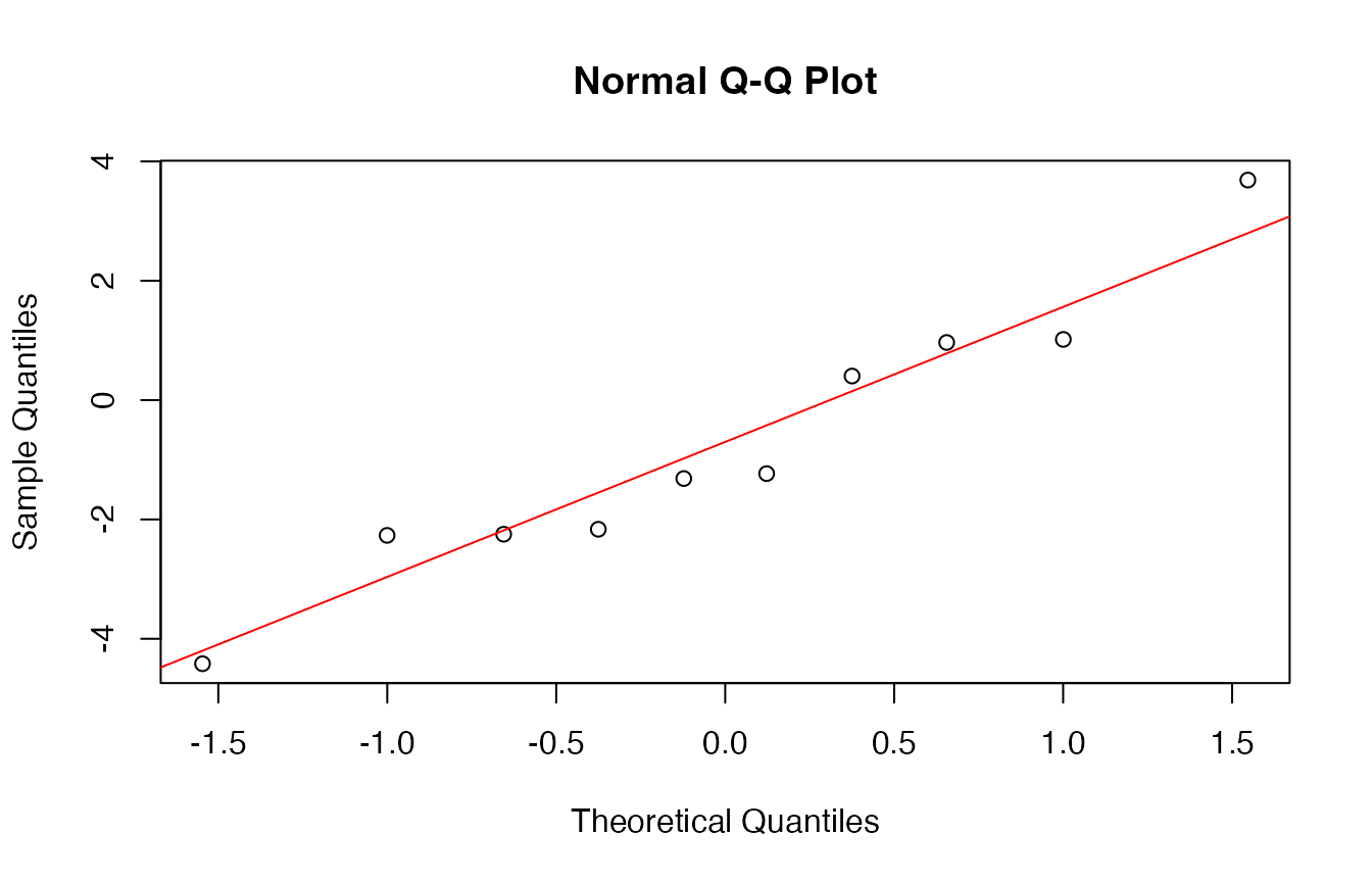
##
##  Shapiro-Wilk normality test
##
## data:  y_test - y_pred
## W = 0.95305, p-value = 0.7047
# -------------------------
# Sparsity diagnostics
# -------------------------
(coef_min <- coef(cv_model, s = "lambda.min"))
## 61 x 1 sparse Matrix of class "dgCMatrix"
##                lambda.min
## (Intercept) 23.5765429179
## cyl         -0.5337018266
## disp        -0.0016855389
## hp          -0.0005736031
## drat         1.3381501299
## wt          -1.4833970316
## qsec         .
## vs           0.8265475926
## am           0.0327132634
## gear         .
## carb         .
## H1           .
## H2          -0.1772888513
## H3           .
## H4          -0.4539984869
## H5           .
## H6           0.0054760046
## H7           .
## H8           .
## H9           .
## H10          .
## H11          .
## H12          .
## H13          .
## H14          .
## H15          .
## H16          .
## H17          .
## H18          .
## H19          .
## H20          .
## H21          .
## H22          .
## H23          .
## H24          .
## H25          .
## H26          .
## H27          .
## H28          .
## H29         -0.9274954853
## H30          .
## H31          .
## H32          .
## H33         -0.7038716722
## H34          .
## H35         -0.0962991954
## H36          .
## H37         -0.4199869874
## H38          .
## H39          .
## H40          .
## H41          .
## H42          .
## H43          .
## H44          .
## H45          .
## H46          .
## H47          .
## H48          .
## H49          .
## H50          .
nonzero <- sum(coef_min[-1, 1] != 0)
cat("Non-zero coefficients:", nonzero, "\n")
## Non-zero coefficients: 14
# Optional: inspect how many come from original vs hidden
p <- ncol(X_train)
orig_nz <- sum(coef_min[2:(p+1), 1] != 0)
hidden_nz <- sum(coef_min[(p+2):length(coef_min), 1] != 0)

cat("Original features used:", orig_nz, "\n")
## Original features used: 7
cat("Hidden features used:", hidden_nz, "\n")
## Hidden features used: 7
2 - 1 Binary classification
set.seed(123)

data(iris)

# Binary classification: setosa vs others
y <- ifelse(iris$Species == "setosa", 1, 0)
X <- as.matrix(iris[, 1:4])

# Train/test split
n <- nrow(X)
idx <- sample(1:n, size = round(0.8 * n))

X_train <- X[idx, ]
y_train <- y[idx]

X_test <- X[-idx, ]
y_test <- y[-idx]

# -------------------------
# Fit model
# -------------------------
cv_model <- cv.rvflnet(
  X_train, y_train,
  n_hidden = 50,
  activation = "relu",
  W_type = "gaussian",
  family = "binomial",
  nfolds = 5
)

# -------------------------
# Predictions (probabilities)
# -------------------------
(probs <- predict(cv_model, X_test, type = "response"))
##         lambda.min
##  [1,] 0.9997617002
##  [2,] 0.9992267955
##  [3,] 0.9997120678
##  [4,] 0.9997524867
##  [5,] 0.9996600481
##  [6,] 0.9992472082
##  [7,] 0.9996101744
##  [8,] 0.9999356520
##  [9,] 0.9998139568
## [10,] 0.9995418762
## [11,] 0.0003328885
## [12,] 0.0003328885
## [13,] 0.0003328885
## [14,] 0.0019937012
## [15,] 0.0003328885
## [16,] 0.0005459970
## [17,] 0.0003328885
## [18,] 0.0005035848
## [19,] 0.0003328885
## [20,] 0.0003328885
## [21,] 0.0003328885
## [22,] 0.0003328885
## [23,] 0.0003328885
## [24,] 0.0003328885
## [25,] 0.0003328885
## [26,] 0.0003328885
## [27,] 0.0003328885
## [28,] 0.0003328885
## [29,] 0.0003328885
## [30,] 0.0003328885
## [1] TRUE
# -------------------------
# Diagnostics
# -------------------------

# Accuracy
acc <- mean(drop(y_pred) == y_test)
cat("Accuracy:", acc, "\n")
## Accuracy: 1
# Confusion matrix
table(Predicted = y_pred, Actual = y_test)
##          Actual
## Predicted  0  1
##         0 20  0
##         1  0 10
# ROC-style diagnostic (simple)
plot(probs, jitter(y_test),
     main = "Predicted probabilities vs true labels",
     xlab = "Predicted probability",
     ylab = "True label")

# Sparsity
(coef_min <- coef(cv_model, s = "lambda.min"))
## 55 x 1 sparse Matrix of class "dgCMatrix"
##               lambda.min
## (Intercept)  -8.00737002
## Sepal.Length  .
## Sepal.Width   .
## Petal.Length  .
## Petal.Width   .
## H1            .
## H2            .
## H3            .
## H4            .
## H5            .
## H6            .
## H7            .
## H8            .
## H9            4.93563803
## H10           .
## H11           .
## H12           .
## H13           .
## H14           .
## H15           .
## H16           .
## H17           .
## H18           .
## H19           .
## H20           .
## H21           .
## H22           .
## H23           .
## H24           .
## H25           .
## H26           .
## H27           .
## H28           .
## H29           .
## H30           .
## H31           .
## H32           .
## H33           .
## H34           .
## H35           .
## H36           0.95999955
## H37           .
## H38           .
## H39           .
## H40           .
## H41           .
## H42           .
## H43           .
## H44           .
## H45           .
## H46           0.05947803
## H47           .
## H48           .
## H49           0.16394482
## H50           .
cat("Non-zero coefficients:", sum(coef_min[-1, 1] != 0), "\n")
## Non-zero coefficients: 4
2 - 2 multiclass classification
set.seed(123)

data(iris)

X <- as.matrix(iris[, 1:4])
y <- as.integer(iris$Species)  # factor with 3 classes

# Train/test split
n <- nrow(X)
idx <- sample(1:n, size = round(0.8 * n))

X_train <- X[idx, ]
y_train <- y[idx]

X_test <- X[-idx, ]
y_test <- y[-idx]

# -------------------------
# Fit model
# -------------------------
cv_model <- cv.rvflnet(
  X_train, y_train,
  n_hidden = 60,
  activation = "tanh",
  W_type = "sobol",
  family = "multinomial",
  nfolds = 5
)

# -------------------------
# Predictions
# -------------------------
(probs <- predict(cv_model, X_test, type = "response"))
## , , lambda.min
##
##                  1            2            3
##  [1,] 9.982426e-01 1.757448e-03 3.459054e-19
##  [2,] 9.932314e-01 6.768590e-03 3.692295e-17
##  [3,] 9.979165e-01 2.083541e-03 3.900101e-18
##  [4,] 9.982099e-01 1.790113e-03 1.432764e-19
##  [5,] 9.979199e-01 2.080148e-03 1.018286e-18
##  [6,] 9.961312e-01 3.868773e-03 1.353780e-18
##  [7,] 9.973898e-01 2.610184e-03 7.426400e-19
##  [8,] 9.996859e-01 3.140579e-04 7.420564e-21
##  [9,] 9.975841e-01 2.415874e-03 1.228506e-18
## [10,] 9.976419e-01 2.358056e-03 1.011165e-17
## [11,] 2.242645e-04 9.616819e-01 3.809380e-02
## [12,] 1.238235e-03 9.822014e-01 1.656038e-02
## [13,] 9.888395e-04 9.758578e-01 2.315332e-02
## [14,] 3.704532e-02 9.629517e-01 2.931757e-06
## [15,] 3.937507e-04 9.970431e-01 2.563106e-03
## [16,] 5.404109e-03 9.945865e-01 9.371371e-06
## [17,] 2.844270e-03 9.928376e-01 4.318177e-03
## [18,] 2.037723e-02 9.795792e-01 4.360441e-05
## [19,] 9.372272e-04 9.985428e-01 5.199913e-04
## [20,] 3.624663e-03 9.962681e-01 1.072695e-04
## [21,] 1.062615e-04 9.744471e-01 2.544661e-02
## [22,] 4.463536e-03 9.953878e-01 1.486454e-04
## [23,] 5.914594e-06 7.729005e-02 9.227040e-01
## [24,] 1.482716e-03 9.975321e-01 9.852118e-04
## [25,] 3.552658e-03 9.951492e-01 1.298191e-03
## [26,] 4.980522e-10 8.255886e-05 9.999174e-01
## [27,] 2.572022e-08 2.481971e-03 9.975180e-01
## [28,] 3.331262e-08 1.779771e-03 9.982202e-01
## [29,] 3.806263e-10 5.416406e-04 9.994584e-01
## [30,] 8.189773e-10 1.072764e-04 9.998927e-01
# Convert probabilities to class
#(pred_class <- apply(probs, 1, function(row) colnames(probs)[which.max(row)]))
(pred_class <- predict(cv_model, X_test, type = "class"))
##       lambda.min
##  [1,] "1"
##  [2,] "1"
##  [3,] "1"
##  [4,] "1"
##  [5,] "1"
##  [6,] "1"
##  [7,] "1"
##  [8,] "1"
##  [9,] "1"
## [10,] "1"
## [11,] "2"
## [12,] "2"
## [13,] "2"
## [14,] "2"
## [15,] "2"
## [16,] "2"
## [17,] "2"
## [18,] "2"
## [19,] "2"
## [20,] "2"
## [21,] "2"
## [22,] "2"
## [23,] "3"
## [24,] "2"
## [25,] "2"
## [26,] "3"
## [27,] "3"
## [28,] "3"
## [29,] "3"
## [30,] "3"
# -------------------------
# Diagnostics
# -------------------------

# Accuracy
acc <- mean(pred_class == y_test)
cat("Accuracy:", acc, "\n")
## Accuracy: 0.9666667
# Confusion matrix
table(Predicted = pred_class, Actual = y_test)
##          Actual
## Predicted  1  2  3
##         1 10  0  0
##         2  0 14  0
##         3  0  1  5
# Sparsity (note: multinomial returns list per class)
(coef_min <- coef(cv_model, s = "lambda.min"))
## $`1`
## 65 x 1 sparse Matrix of class "dgCMatrix"
##              lambda.min
## (Intercept)   16.512314
## Sepal.Length   .
## Sepal.Width    3.251664
## Petal.Length  -2.602282
## Petal.Width   -1.688998
## H1             .
## H2             .
## H3             .
## H4             .
## H5             .
## H6             .
## H7             .
## H8             .
## H9             .
## H10            .
## H11            .
## H12            .
## H13            .
## H14            .
## H15            .
## H16            .
## H17            .
## H18            .
## H19            .
## H20            .
## H21            .
## H22            .
## H23            .
## H24            .
## H25            .
## H26            .
## H27            .
## H28            .
## H29            .
## H30            .
## H31            .
## H32            .
## H33            .
## H34            .
## H35            .
## H36            .
## H37            .
## H38            .
## H39            .
## H40            .
## H41            .
## H42            .
## H43            .
## H44            .
## H45            .
## H46            .
## H47            .
## H48            .
## H49            .
## H50            .
## H51            .
## H52            .
## H53            .
## H54            .
## H55            .
## H56            .
## H57            .
## H58            .
## H59            .
## H60            .
##
## $`2`
## 65 x 1 sparse Matrix of class "dgCMatrix"
##              lambda.min
## (Intercept)   10.624601
## Sepal.Length   1.361845
## Sepal.Width    .
## Petal.Length   .
## Petal.Width    .
## H1             .
## H2             .
## H3             .
## H4             .
## H5             .
## H6             .
## H7             .
## H8             .
## H9             .
## H10            .
## H11            .
## H12            .
## H13            .
## H14            .
## H15            .
## H16            .
## H17            .
## H18            .
## H19            .
## H20            .
## H21            .
## H22            .
## H23            .
## H24            .
## H25            .
## H26            .
## H27            .
## H28            .
## H29            .
## H30            .
## H31            .
## H32            .
## H33            .
## H34            .
## H35            .
## H36            .
## H37            .
## H38            .
## H39            .
## H40            .
## H41            .
## H42            .
## H43            .
## H44            .
## H45            .
## H46            .
## H47            .
## H48            .
## H49            .
## H50            .
## H51            .
## H52            .
## H53            .
## H54            .
## H55            .
## H56            .
## H57            .
## H58            .
## H59            .
## H60            .
##
## $`3`
## 65 x 1 sparse Matrix of class "dgCMatrix"
##               lambda.min
## (Intercept)  -27.1369151
## Sepal.Length   .
## Sepal.Width    .
## Petal.Length   6.0134319
## Petal.Width    9.7916675
## H1             .
## H2             .
## H3             .
## H4             .
## H5             .
## H6             .
## H7             0.8319143
## H8             .
## H9             .
## H10            .
## H11            .
## H12            .
## H13            .
## H14            .
## H15            .
## H16            .
## H17            .
## H18            .
## H19            .
## H20            .
## H21            .
## H22            .
## H23            .
## H24            .
## H25            .
## H26            .
## H27            .
## H28            .
## H29            .
## H30            .
## H31            .
## H32            .
## H33            .
## H34            .
## H35            .
## H36            .
## H37            .
## H38            .
## H39            .
## H40            .
## H41            .
## H42            .
## H43            .
## H44            .
## H45            .
## H46            .
## H47            .
## H48            .
## H49            .
## H50            .
## H51           -2.9870762
## H52            .
## H53            .
## H54            .
## H55            .
## H56            .
## H57            .
## H58            .
## H59            .
## H60            .