## Loading required package: ggplot2
## Loading required package: gridExtra
## Loading required package: reshape2
## Loading required package: VineCopula
## Loading required package: randtoolbox
## Loading required package: rngWELL
## This is randtoolbox. For an overview, type 'help("randtoolbox")'.
## Loading required package: zoo
##
## Attaching package: 'zoo'
## The following objects are masked from 'package:base':
##
##     as.Date, as.Date.numeric
## Loading required package: data.table
##
## Attaching package: 'data.table'
## The following objects are masked from 'package:zoo':
##
##     yearmon, yearqtr
## The following objects are masked from 'package:reshape2':
##
##     dcast, melt
##
##
##  This is version 1.10.2 of esgtoolkit. Starting with 1.0.0, package renamed as: 'esgtoolkit' (lowercase)
##
##
y <- EuStockMarkets[1:250, ]

# Run simulation
result <- simulate_rvine(y, n = 300, verbose = TRUE, n_trials = 5)
## Transforming data to uniform margins with improved boundary handling...
## Fitting R-vine copula model...
## V1 + V3 --> V1,V3 ; V2
## V2 + V4 --> V2,V4 ; V3
## V1 + V4 --> V1,V4 ; V3,V2
## R-vine copula model fitted successfully
## tree     edge | family   cop    par  par2 |  tau   utd   ltd
## ------------------------------------------------------------
##    1      2,1 |      5     F  16.91  0.00 | 0.79     -     -
##           3,2 |      9   BB7   4.18  1.74 | 0.70  0.82  0.67
##           4,3 |     19  SBB7   1.80  1.26 | 0.50  0.58  0.53
##    2    3,1;2 |      2     t   0.18  2.74 | 0.11  0.19  0.19
##         4,2;3 |     13    SC   0.23  0.00 | 0.10  0.05     -
##    3  4,1;3,2 |     13    SC   0.20  0.00 | 0.09  0.03     -
## ---
## type: D-vine    logLik: 595.34    AIC: -1172.68    BIC: -1140.99
## ---
## 1 <-> V1,   2 <-> V2,   3 <-> V3,   4 <-> V4  tree    edge family  cop        par     par2        tau        utd       ltd
## 1    1     4,3     19 SBB7  1.8013403 1.256235 0.50242484 0.57593221 0.5306866
## 2    1     3,2      9  BB7  4.1797300 1.740122 0.70055786 0.81962121 0.6714387
## 3    1     2,1      5    F 16.9079788 0.000000 0.78638157 0.00000000 0.0000000
## 4    2   4,2;3     13   SC  0.2309033 0.000000 0.10350217 0.04969290 0.0000000
## 5    2   3,1;2      2    t  0.1759103 2.740196 0.11257372 0.18566694 0.1856669
## 6    3 4,1;3,2     13   SC  0.1974467 0.000000 0.08985277 0.02988036 0.0000000
## Running 5 simulation trials...
## Best simulation achieved quality score: 0.0363
## Score weights used: [0.4, 0.2, 0.2, 0.1, 0.1]
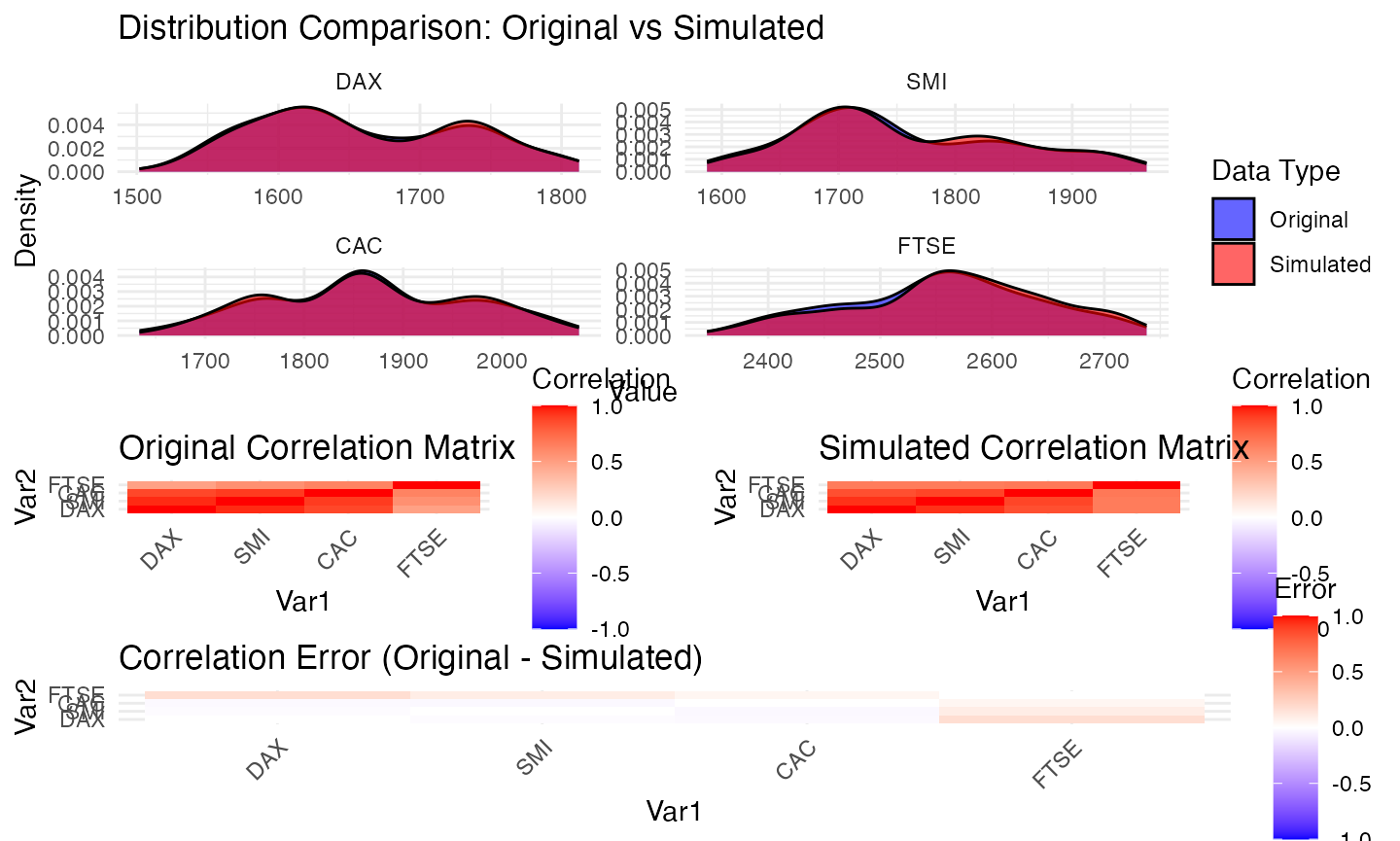
## Mean absolute correlation error (Kendall): 0.0415
## Mean absolute correlation error (Pearson): 0.0489
# Print summary
print(result)
## R-vine Copula Simulation Results
## ================================
##
## Original observations: 250
## Variables: 4
## Simulated observations: 300
## Quality score: 0.0363
## Successful trials: 5/5
## Mean absolute correlation error (Kendall): 0.0415
## Mean absolute correlation error (Pearson): 0.0489
##
## Use plot() to visualize results and $diagnostics for detailed metrics.
# Create different types of plots
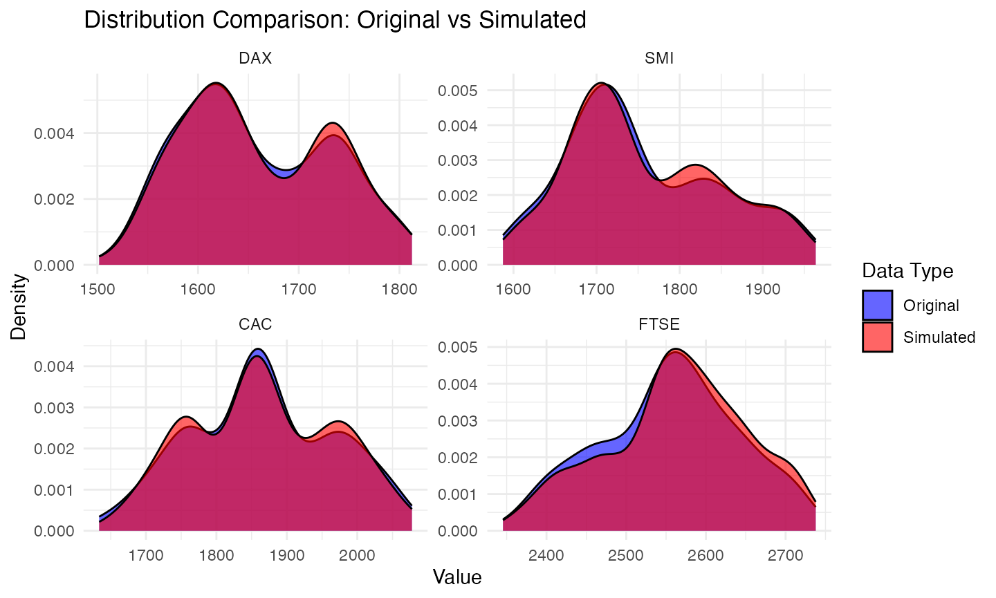
plot(result, type = "distribution") # Default
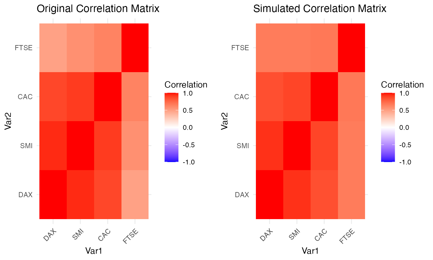
plot(result, type = "correlation")
plot(result, type = "both")

# Access detailed diagnostics
str(result$diagnostics)
## List of 24
##  $ original_correlation_tau     : num [1:4, 1:4] 1 0.801 0.67 0.333 0.801 ...
##   ..- attr(*, "dimnames")=List of 2
##   .. ..$ : chr [1:4] "DAX" "SMI" "CAC" "FTSE"
##   .. ..$ : chr [1:4] "DAX" "SMI" "CAC" "FTSE"
##  $ simulated_correlation_tau    : num [1:4, 1:4] 1 0.8 0.666 0.474 0.8 ...
##   ..- attr(*, "dimnames")=List of 2
##   .. ..$ : chr [1:4] "DAX" "SMI" "CAC" "FTSE"
##   .. ..$ : chr [1:4] "DAX" "SMI" "CAC" "FTSE"
##  $ correlation_error_tau        : num [1:4, 1:4] 0 -0.000753 -0.004057 0.140903 -0.000753 ...
##   ..- attr(*, "dimnames")=List of 2
##   .. ..$ : chr [1:4] "DAX" "SMI" "CAC" "FTSE"
##   .. ..$ : chr [1:4] "DAX" "SMI" "CAC" "FTSE"
##  $ original_correlation_pearson : num [1:4, 1:4] 1 0.95 0.87 0.486 0.95 ...
##   ..- attr(*, "dimnames")=List of 2
##   .. ..$ : chr [1:4] "DAX" "SMI" "CAC" "FTSE"
##   .. ..$ : chr [1:4] "DAX" "SMI" "CAC" "FTSE"
##  $ simulated_correlation_pearson: num [1:4, 1:4] 1 0.934 0.844 0.661 0.934 ...
##   ..- attr(*, "dimnames")=List of 2
##   .. ..$ : chr [1:4] "DAX" "SMI" "CAC" "FTSE"
##   .. ..$ : chr [1:4] "DAX" "SMI" "CAC" "FTSE"
##  $ correlation_error_pearson    : num [1:4, 1:4] 0 -0.016 -0.0261 0.1752 -0.016 ...
##   ..- attr(*, "dimnames")=List of 2
##   .. ..$ : chr [1:4] "DAX" "SMI" "CAC" "FTSE"
##   .. ..$ : chr [1:4] "DAX" "SMI" "CAC" "FTSE"
##  $ mean_absolute_error_tau      : num 0.0415
##  $ max_absolute_error_tau       : num 0.141
##  $ mean_absolute_error_pearson  : num 0.0489
##  $ max_absolute_error_pearson   : num 0.175
##  $ quality_score                : num 0.0363
##  $ score_weights_used           : num [1:5] 0.4 0.2 0.2 0.1 0.1
##  $ trial_scores                 : num [1:5] 0.0401 0.0482 0.0381 0.0363 0.0546
##  $ successful_trials            : int 5
##  $ RVM_model                    :List of 20
##   ..$ Matrix     : num [1:4, 1:4] 1 4 3 2 0 2 4 3 0 0 ...
##   ..$ family     : num [1:4, 1:4] 0 13 2 5 0 0 13 9 0 0 ...
##   ..$ par        : num [1:4, 1:4] 0 0.197 0.176 16.908 0 ...
##   ..$ par2       : num [1:4, 1:4] 0 0 2.74 0 0 ...
##   ..$ names      : chr [1:4] "V1" "V2" "V3" "V4"
##   ..$ MaxMat     : num [1:4, 1:4] 1 2 2 2 0 2 3 3 0 0 ...
##   ..$ CondDistr  :List of 2
##   .. ..$ direct  : logi [1:4, 1:4] FALSE TRUE TRUE TRUE FALSE FALSE ...
##   .. ..$ indirect: logi [1:4, 1:4] FALSE FALSE FALSE FALSE FALSE TRUE ...
##   ..$ type       : chr "D-vine"
##   ..$ tau        : num [1:4, 1:4] 0 0.0899 0.1126 0.7864 0 ...
##   ..$ taildep    :List of 2
##   .. ..$ upper: num [1:4, 1:4] 0 0.0299 0.1857 0 0 ...
##   .. ..$ lower: num [1:4, 1:4] 0 0 0.186 0 0 ...
##   ..$ beta       : num [1:4, 1:4] 0 0.0871 NA 0.8361 0 ...
##   ..$ call       : language VineCopula::RVineStructureSelect(data = U, familyset = valid_families,      type = 0, selectioncrit = "BIC", trun| __truncated__ ...
##   ..$ nobs       : int 250
##   ..$ logLik     : num 595
##   ..$ pair.logLik: num [1:4, 1:4] 0 2.81 12.84 258.25 0 ...
##   ..$ AIC        : num -1173
##   ..$ pair.AIC   : num [1:4, 1:4] 0 -3.63 -21.68 -514.51 0 ...
##   ..$ BIC        : num -1141
##   ..$ pair.BIC   : num [1:4, 1:4] 0 -0.105 -14.638 -510.985 0 ...
##   ..$ emptau     : num [1:4, 1:4] 0 0.066 0.112 0.801 0 ...
##   ..- attr(*, "class")= chr "RVineMatrix"
##  $ n_observations               : int 250
##  $ n_variables                  : int 4
##  $ n_simulations                : num 300
##  $ original_means               : Named num [1:4] 1658 1756 1865 2555
##   ..- attr(*, "names")= chr [1:4] "DAX" "SMI" "CAC" "FTSE"
##  $ simulated_means              : Named num [1:4] 1660 1759 1866 2564
##   ..- attr(*, "names")= chr [1:4] "DAX" "SMI" "CAC" "FTSE"
##  $ original_sds                 : Named num [1:4] 73.5 92.6 102.3 87.2
##   ..- attr(*, "names")= chr [1:4] "DAX" "SMI" "CAC" "FTSE"
##  $ simulated_sds                : Named num [1:4] 73.7 91.2 101.1 87.7
##   ..- attr(*, "names")= chr [1:4] "DAX" "SMI" "CAC" "FTSE"
##  $ ks_test_statistics           : Named num [1:4] 0.0327 0.042 0.0347 0.068
##   ..- attr(*, "names")= chr [1:4] "D" "D" "D" "D"
##  $ ks_test_pvalues              : num [1:4] 0.999 0.97 0.997 0.554
# Access simulated data
sim_data <- result$simulated_data

head(sim_data)
##           DAX      SMI      CAC     FTSE
## [1,] 1605.796 1670.100 1776.371 2515.914
## [2,] 1686.930 1840.530 1888.391 2594.548
## [3,] 1717.650 1838.949 1856.796 2544.001
## [4,] 1591.506 1699.128 1759.658 2423.380
## [5,] 1649.241 1723.023 1840.551 2525.274
## [6,] 1646.024 1732.583 1832.104 2463.487