Model-agnostic statistical probabilistic forecasting with conditional volatility

Combines a mean model and a volatility model to produce probabilistic forecasts. Uncertainty is propagated from two sources: simulated innovation draws and simulated volatility paths derived from the variance model's residuals via bootstrap.

condvolf(
  y,
  h = 10L,
  mean_model = forecast::auto.arima,
  sigma_model = forecast::auto.arima,
  innovation = c("empirical", "gaussian", "student"),
  level = 95,
  B = 1000L,
  bootstrap_vol = TRUE,
  ...
)

Arguments

y: A numeric vector or time series of class ts.
h: Forecasting horizon.
mean_model: Function to fit the mean model (default: forecast::auto.arima). Options include forecast::auto.arima, forecast::ets, forecast::thetaf, or any custom function that returns an object with forecast method.
sigma_model: Function to fit the variance model on squared residuals (default: forecast::auto.arima).
innovation: Distribution for standardized innovations. One of "gaussian" (fastest, often sufficient), "student" (heavy-tailed), or "empirical" (non-parametric, most flexible).
level: Confidence level for prediction intervals (default: 95).
B: Number of simulated paths (default: 2000).
bootstrap_vol: Whether to bootstrap volatility residuals (default: TRUE). If FALSE, uses parametric normal approximation for volatility.
...: Additional arguments passed to mean_model and sigma_model.

Value

A forecast object with components:

x: Original time series.
mean: Point forecast (mean of simulations).
lower: Lower prediction interval bound.
upper: Upper prediction interval bound.
level: Confidence level.
sims: Matrix of simulated forecast paths (h x B).
model: List containing mean and sigma model fits.
residuals: Residuals from the mean model.
standardized_residuals: Scaled standardized residuals used for innovation fitting.
method: Character string describing the method used.

Examples

# \donttest{
library(forecast)

# Basic usage with Google stock data
y <- fpp2::goog200

# Gaussian innovations (fastest, often sufficient)
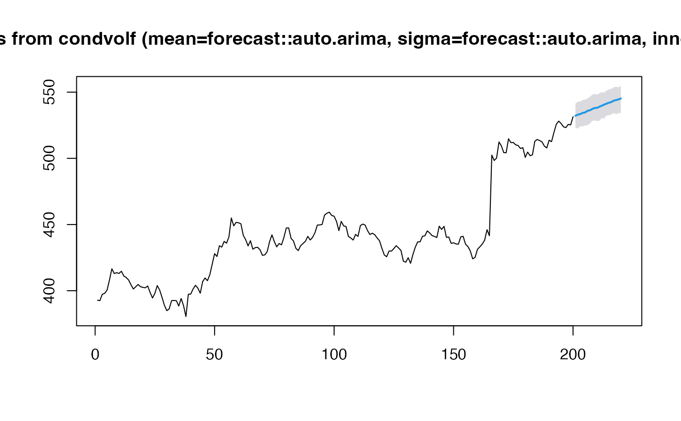
fc1 <- condvolf(y, h = 20, innovation = "gaussian")
plot(fc1)


# Student-t innovations (heavy-tailed)
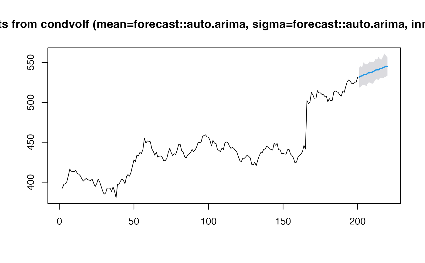
fc2 <- condvolf(y, h = 20, innovation = "student")
#> Warning: NaNs produced
plot(fc2)


# Empirical innovations (non-parametric)
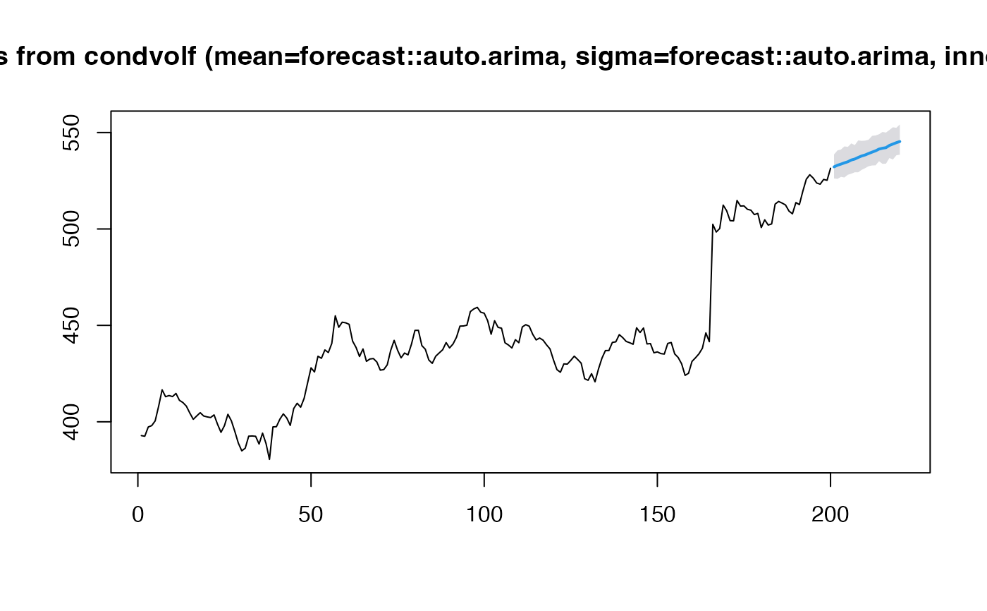
fc3 <- condvolf(y, h = 20, innovation = "empirical")
plot(fc3)


# Using different mean and volatility models
fc4 <- condvolf(y, h = 20,
                mean_model = forecast::thetaf,
                sigma_model = forecast::ets,
                innovation = "gaussian")

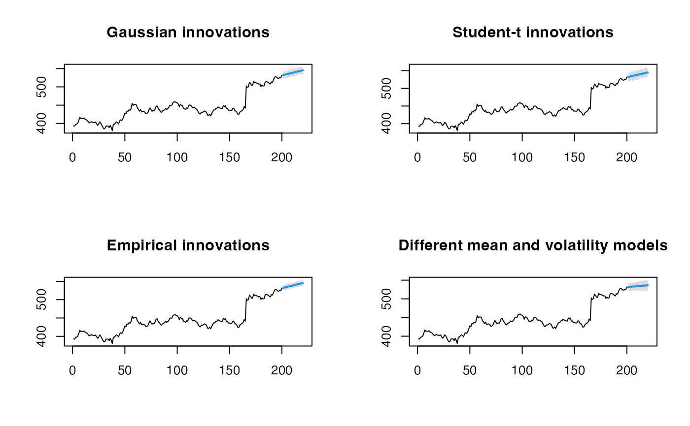
# Compare prediction intervals
par(mfrow = c(2, 2))
plot(fc1, main = "Gaussian innovations")
plot(fc2, main = "Student-t innovations")
plot(fc3, main = "Empirical innovations")
plot(fc4, main = "Different mean and volatility models")

par(mfrow = c(1, 1))
# }